The following application is inspired by the empirical example in “Measuring the model risk-adjusted performance of machine learning algorithms in credit default prediction” by Alonso Robisco and Carbó Martínez (2022). However, since we are not interested in model risk-adjusted performance, the application will purely focus on the implementation of machine learning algorithms for loan default prediction.
6.1 Problem Setup
The dataset that we will be using was used in the Kaggle competition “Give Me Some Credit”. The description of the competition reads as follows:
Banks play a crucial role in market economies. They decide who can get finance and on what terms and can make or break investment decisions. For markets and society to function, individuals and companies need access to credit.
Credit scoring algorithms, which make a guess at the probability of default, are the method banks use to determine whether or not a loan should be granted. This competition requires participants to improve on the state of the art in credit scoring, by predicting the probability that somebody will experience financial distress in the next two years.
The goal of this competition is to build a model that borrowers can use to help make the best financial decisions.
Historical data are provided on 250,000 borrowers and the prize pool is $5,000 ($3,000 for first, $1,500 for second and $500 for third).
Unfortunately, there won’t be any prize money today. However, the experience that you can gain from working through an application like this can be invaluable. So, in a way, you are still winning!
6.2 Dataset
Let’s download the dataset automatically, unzip it, and place it in a folder called data if you haven’t done so already
from io import BytesIOfrom urllib.request import urlopenfrom zipfile import ZipFileimport os.path# Check if the file existsifnot os.path.isfile('data/Data Dictionary.xl') ornot os.path.isfile('data/cs-training.csv'):print('Downloading dataset...')# Define the dataset to be downloaded zipurl ='https://www.kaggle.com/api/v1/datasets/download/brycecf/give-me-some-credit-dataset'# Download and unzip the dataset in the data folderwith urlopen(zipurl) as zipresp:with ZipFile(BytesIO(zipresp.read())) as zfile: zfile.extractall('data')print('DONE!')else:print('Dataset already downloaded!')
Downloading dataset...
DONE!
Then, we can have a look at the data dictionary that is provided with the dataset. This will give us an idea of the variables that are available in the dataset and what they represent
import pandas as pddata_dict = pd.read_excel('data/Data Dictionary.xls', header=1)data_dict.style.hide()
Variable Name
Description
Type
SeriousDlqin2yrs
Person experienced 90 days past due delinquency or worse
Y/N
RevolvingUtilizationOfUnsecuredLines
Total balance on credit cards and personal lines of credit except real estate and no installment debt like car loans divided by the sum of credit limits
percentage
age
Age of borrower in years
integer
NumberOfTime30-59DaysPastDueNotWorse
Number of times borrower has been 30-59 days past due but no worse in the last 2 years.
integer
DebtRatio
Monthly debt payments, alimony,living costs divided by monthy gross income
percentage
MonthlyIncome
Monthly income
real
NumberOfOpenCreditLinesAndLoans
Number of Open loans (installment like car loan or mortgage) and Lines of credit (e.g. credit cards)
integer
NumberOfTimes90DaysLate
Number of times borrower has been 90 days or more past due.
integer
NumberRealEstateLoansOrLines
Number of mortgage and real estate loans including home equity lines of credit
integer
NumberOfTime60-89DaysPastDueNotWorse
Number of times borrower has been 60-89 days past due but no worse in the last 2 years.
integer
NumberOfDependents
Number of dependents in family excluding themselves (spouse, children etc.)
integer
The variable \(y\) that we want to predict is SeriousDlqin2yrs which indicates whether a person has been 90 days past due on a loan payment (serious delinquency) in the past two years. This target variable is \(1\) if the loan defaults (i.e., serious delinquency occured) and \(0\) if the loan does not default (i.e., no serious delinquency occured) . The other variables are features that we can use to predict this target variable such as the age of the borrower and the monthly income of the borrower.
6.3 Putting the Problem into the Context of the Course
Given the description of the competition and the dataset, we can see that this is a supervised learning problem. We have a target variable that we want to predict, and we have features that we can use to predict this target variable. The target variable is binary, i.e., it can take two values: 0 or 1. The value 0 indicates that the loan will not default, while the value 1 indicates that the loan will default. Thus, this is a binary classification problem.
6.4 Setting up the Environment
We will start by setting up the environment by importing the necessary libraries
import numpy as npimport pandas as pdimport matplotlib.pyplot as pltimport seaborn as sns
and loading the dataset
df = pd.read_csv('data/cs-training.csv')
Let’s also download some precomputed models that we will use later on
for file_name in ['clf_nn.joblib', 'clf_nn2.joblib']:ifnot os.path.isfile(file_name):print(f'Downloading {file_name}...')# Generate the download link url =f'https://github.com/jmarbet/data-science-course/raw/main/notebooks/{file_name}'# Download the filewith urlopen(url) as response, open(file_name, 'wb') as out_file: data = response.read() out_file.write(data)print('DONE!')else:print(f'{file_name} already downloaded!')
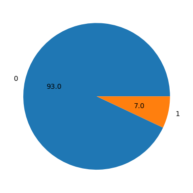
Note that the column MonthlyIncome and NumberOfDependents seem to have missing values. Before we drop these missing values or impute them, let’s have a look at the distribution of our target variable SeriousDlqin2yrs
As with the example that we have seen during one of our previous lectures, the dataset seems to be quite imbalanced. Only about 6.7% of the loans have defaulted. This is something that we need to keep in mind when treating the missing values and when building our models.
Let’s see what happens to the distribution of the target variable if we drop the missing values
It seems to have almost no impact on the distribution of the target variable. This is good news. Let’s compare some other statistics of the dataset before and after dropping the missing values
df.describe().T
count
mean
std
min
25%
50%
75%
max
SeriousDlqin2yrs
150000.0
0.066840
0.249746
0.0
0.000000
0.000000
0.000000
1.0
age
150000.0
52.295207
14.771866
0.0
41.000000
52.000000
63.000000
109.0
NumberOfDependents
146076.0
0.757222
1.115086
0.0
0.000000
0.000000
1.000000
20.0
MonthlyIncome
120269.0
6670.221237
14384.674215
0.0
3400.000000
5400.000000
8249.000000
3008750.0
DebtRatio
150000.0
353.005076
2037.818523
0.0
0.175074
0.366508
0.868254
329664.0
RevolvingUtilizationOfUnsecuredLines
150000.0
6.048438
249.755371
0.0
0.029867
0.154181
0.559046
50708.0
NumberOfOpenCreditLinesAndLoans
150000.0
8.452760
5.145951
0.0
5.000000
8.000000
11.000000
58.0
NumberRealEstateLoansOrLines
150000.0
1.018240
1.129771
0.0
0.000000
1.000000
2.000000
54.0
NumberOfTime30-59DaysPastDueNotWorse
150000.0
0.421033
4.192781
0.0
0.000000
0.000000
0.000000
98.0
NumberOfTime60-89DaysPastDueNotWorse
150000.0
0.240387
4.155179
0.0
0.000000
0.000000
0.000000
98.0
NumberOfTimes90DaysLate
150000.0
0.265973
4.169304
0.0
0.000000
0.000000
0.000000
98.0
df.dropna().describe().T
count
mean
std
min
25%
50%
75%
max
SeriousDlqin2yrs
120269.0
0.069486
0.254280
0.0
0.000000
0.000000
0.000000
1.0
age
120269.0
51.289792
14.426684
0.0
40.000000
51.000000
61.000000
103.0
NumberOfDependents
120269.0
0.851832
1.148391
0.0
0.000000
0.000000
2.000000
20.0
MonthlyIncome
120269.0
6670.221237
14384.674215
0.0
3400.000000
5400.000000
8249.000000
3008750.0
DebtRatio
120269.0
26.598777
424.446457
0.0
0.143388
0.296023
0.482559
61106.5
RevolvingUtilizationOfUnsecuredLines
120269.0
5.899873
257.040685
0.0
0.035084
0.177282
0.579428
50708.0
NumberOfOpenCreditLinesAndLoans
120269.0
8.758475
5.172835
0.0
5.000000
8.000000
11.000000
58.0
NumberRealEstateLoansOrLines
120269.0
1.054519
1.149273
0.0
0.000000
1.000000
2.000000
54.0
NumberOfTime30-59DaysPastDueNotWorse
120269.0
0.381769
3.499234
0.0
0.000000
0.000000
0.000000
98.0
NumberOfTime60-89DaysPastDueNotWorse
120269.0
0.187829
3.447901
0.0
0.000000
0.000000
0.000000
98.0
NumberOfTimes90DaysLate
120269.0
0.211925
3.465276
0.0
0.000000
0.000000
0.000000
98.0
It looks like the statistics before and after dropping the missing values are quite similar, except for the variable DebtRatio, where we have substantially lower means and standard deviation. Let’s also have a look at the distribution of the variables for the rows that we have dropped
df.loc[df.isna().any(axis=1)].describe().T
count
mean
std
min
25%
50%
75%
max
SeriousDlqin2yrs
29731.0
0.056137
0.230189
0.0
0.000000
0.000000
0.000000
1.0
age
29731.0
56.362349
15.438786
21.0
46.000000
57.000000
67.000000
109.0
NumberOfDependents
25807.0
0.316310
0.809944
0.0
0.000000
0.000000
0.000000
9.0
MonthlyIncome
0.0
NaN
NaN
NaN
NaN
NaN
NaN
NaN
DebtRatio
29731.0
1673.396556
4248.372895
0.0
123.000000
1159.000000
2382.000000
329664.0
RevolvingUtilizationOfUnsecuredLines
29731.0
6.649421
217.814854
0.0
0.016027
0.081697
0.440549
22198.0
NumberOfOpenCreditLinesAndLoans
29731.0
7.216071
4.842720
0.0
4.000000
6.000000
10.000000
45.0
NumberRealEstateLoansOrLines
29731.0
0.871481
1.034291
0.0
0.000000
1.000000
1.000000
23.0
NumberOfTime30-59DaysPastDueNotWorse
29731.0
0.579866
6.255361
0.0
0.000000
0.000000
0.000000
98.0
NumberOfTime60-89DaysPastDueNotWorse
29731.0
0.452995
6.242076
0.0
0.000000
0.000000
0.000000
98.0
NumberOfTimes90DaysLate
29731.0
0.484612
6.250408
0.0
0.000000
0.000000
0.000000
98.0
Again, the mean of the dropped rows seems to be substantially higher for the variable DebtRatio suggesting that the missing values are not missing entirely at random. Note, however, that the standard deviation is lower meaning that the dropped observations are more similar to each other in the DebtRatio dimension. From our data dictionary, we know that the DebtRatio is defined as
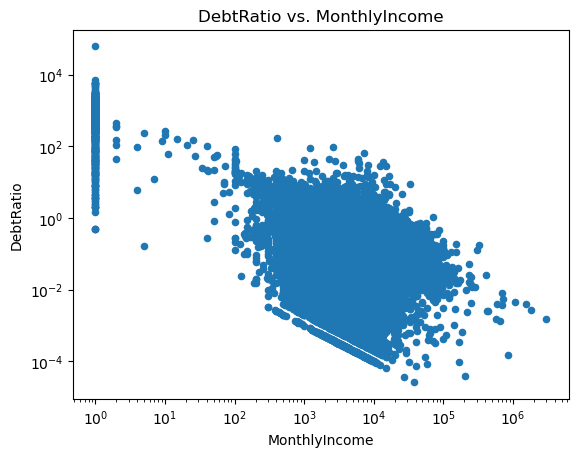
It does not say whether this is in gross or net terms though. Nevertheless, let’s have a look at the relationship between the DebtRatio and the MonthlyIncome
ax = df.plot.scatter(x='MonthlyIncome', y='DebtRatio')ax.set_xscale('log')ax.set_yscale('log')ax.set_xlabel('MonthlyIncome')ax.set_ylabel('DebtRatio')ax.set_title('DebtRatio vs. MonthlyIncome')plt.show()
This looks rather odd. Note how there are a lot of monthly incomes that are close to zero. Furthermore, there is a weird gap going through the scatter points. We can look at the descriptive statistics of the rows with MonthlyIncome less than 100
df.query('MonthlyIncome <= 100').describe().T
count
mean
std
min
25%
50%
75%
max
SeriousDlqin2yrs
2301.0
0.036506
0.187586
0.0
0.000000
0.000000
0.000000
1.0
age
2301.0
47.740113
16.199176
21.0
35.000000
46.000000
60.000000
103.0
NumberOfDependents
2301.0
0.778792
1.192441
0.0
0.000000
0.000000
2.000000
10.0
MonthlyIncome
2301.0
1.837027
11.408271
0.0
0.000000
0.000000
1.000000
100.0
DebtRatio
2301.0
1370.529300
2752.843610
0.0
79.000000
732.000000
1850.500000
61106.5
RevolvingUtilizationOfUnsecuredLines
2301.0
3.604101
125.553453
0.0
0.022243
0.113149
0.486629
5893.0
NumberOfOpenCreditLinesAndLoans
2301.0
7.171230
4.869628
0.0
4.000000
6.000000
10.000000
31.0
NumberRealEstateLoansOrLines
2301.0
0.742721
0.904984
0.0
0.000000
1.000000
1.000000
9.0
NumberOfTime30-59DaysPastDueNotWorse
2301.0
0.549326
6.132226
0.0
0.000000
0.000000
0.000000
98.0
NumberOfTime60-89DaysPastDueNotWorse
2301.0
0.428509
6.124274
0.0
0.000000
0.000000
0.000000
98.0
NumberOfTimes90DaysLate
2301.0
0.438505
6.128357
0.0
0.000000
0.000000
0.000000
98.0
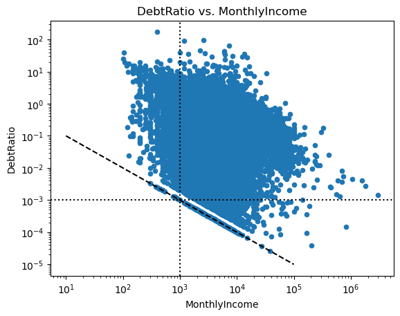
These observations seem to have a higher debtRatio than the rest of the dataset but are less likely to default on their loans (the mean of SeriousDlqin2yrs is equal to the fraction of defaulting loans). Given that they have no income (or essentially no income), this seems rather odd and is likely due to an error during data entry/collection. Since there are only a small number of observations with MonthlyIncome less than 100, we can probably drop them. Let’s look at the same figure for MonthlyIncome greater than 100
This looks better but note how the scatter points below the gap seem to line up with the line \(\frac{1}{\text{MonthlyIncome}}\). Thus, there seems to be another potential data entry/collection error since the debt in the raw data has likely been just set to \(1\) for these observations. If this was a real dataset, we would need to investigate this further and maybe talk to the people who have sent us the data. However, given that this is just an example, we leave it as is.
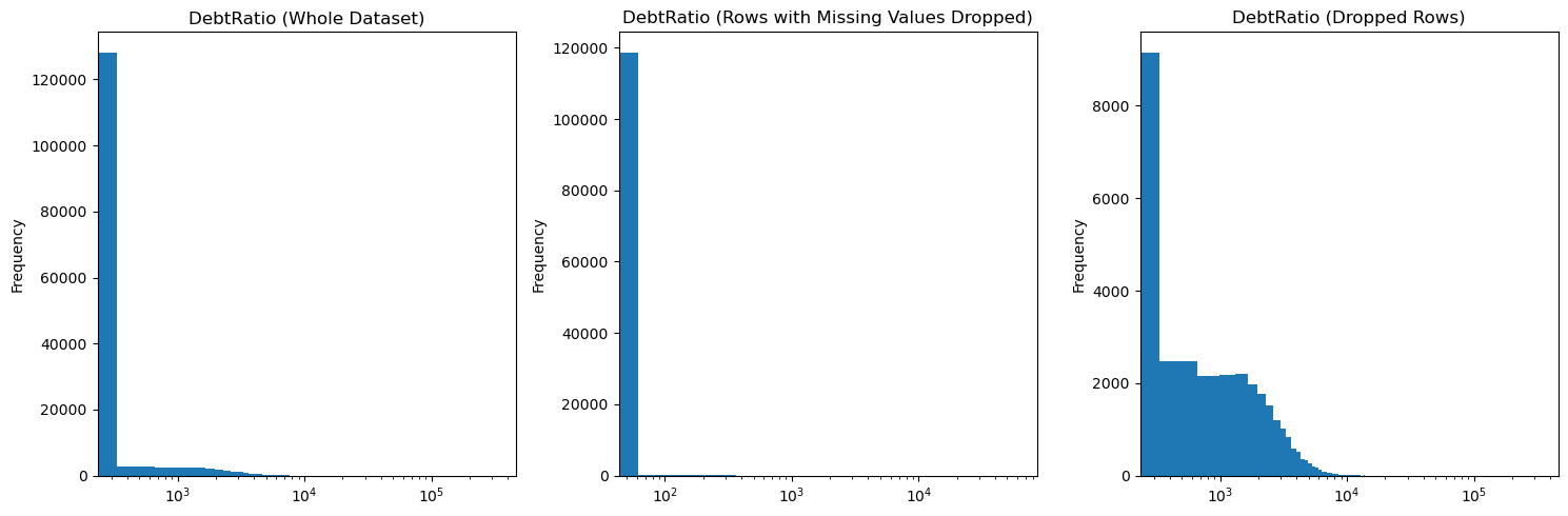
Let’s also have a look at the distribution of DebtRatio variable
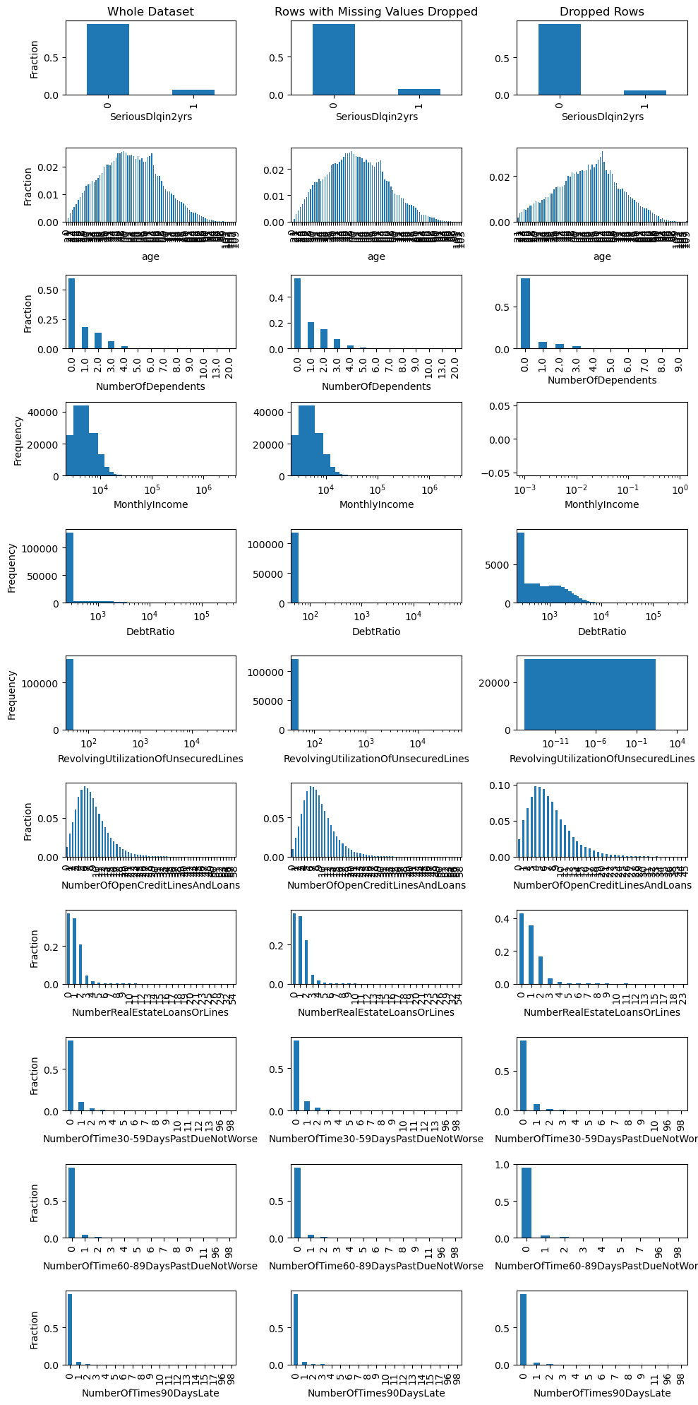
Where we can again see the high DebtRatio values for the rows with missing values. We can also have a look at the distribution of all the variables in the dataset
fig, ax = plt.subplots(df.shape[1], 3, figsize=(10, 20))for ii, col inenumerate(df.columns):# Plot the distribution of the variable for the whole dataset, the dataset with missing values dropped, and the dropped rowsif col in ('SeriousDlqin2yrs', 'age', 'NumberOfTime30-59DaysPastDueNotWorse', 'NumberOfOpenCreditLinesAndLoans', 'NumberOfTimes90DaysLate', 'NumberRealEstateLoansOrLines', 'NumberOfTime60-89DaysPastDueNotWorse', 'NumberOfDependents'): # Use a bar plot for discrete variables df[col].value_counts(normalize=True).sort_index().plot.bar(ax=ax[ii,0]) df.dropna()[col].value_counts(normalize=True).sort_index().plot.bar(ax=ax[ii,1]) df.loc[df.isna().any(axis=1), col].value_counts(normalize=True).sort_index().plot.bar(ax=ax[ii,2])# Set the y-axis label ax[ii,0].set_ylabel('Fraction') ax[ii,1].set_ylabel('') ax[ii,2].set_ylabel('')else:# Use a histogram for continuous variables df[col].plot.hist(bins=1000, ax=ax[ii,0]) df.dropna()[col].plot.hist(bins=1000, ax=ax[ii,1]) df.loc[df.isna().any(axis=1), col].plot.hist(bins=1000, ax=ax[ii,2])# Set the x-axis to a logarithmic scale for the continuous variables ax[ii,0].set_xscale('log') ax[ii,1].set_xscale('log') ax[ii,2].set_xscale('log')# Set the x-axis label ax[ii,0].set_xlabel(col) ax[ii,1].set_xlabel(col) ax[ii,2].set_xlabel(col)# Set the y-axis label ax[ii,0].set_ylabel('Frequency') ax[ii,1].set_ylabel('') ax[ii,2].set_ylabel('')ax[0,0].set_title('Whole Dataset')ax[0,1].set_title('Rows with Missing Values Dropped')ax[0,2].set_title('Dropped Rows')fig.tight_layout()plt.show()
This shows another potential issue with our dataset. Checkout the variable NumberOfTime30-59DaysPastDueNotWorse. It seems that there are a some observations with values greater than 90. This seems rather odd. Let’s have a look at the data dictionary
Number of times borrower has been 30-59 days past due but no worse in the last 2 years.
integer
NumberOfTimes90DaysLate
Number of times borrower has been 90 days or more past due.
integer
NumberOfTime60-89DaysPastDueNotWorse
Number of times borrower has been 60-89 days past due but no worse in the last 2 years.
integer
The data dictionary does not mention anything about values above 90. These values may have a special meaning such as being a flag for missing values. Let’s have a look at the distribution of the target variable for the rows with values greater than 90
There seems to be a very high number of defaults for these observations (more than half), which makes sense given the meaning of these variables. Furthermore, the observations with above 90 in one category have it above 90 in the other categories as well. Thus, this might not be a data entry/collection error and these are just borrowers who commonly fail to make loan payments.
Given that Alonso Robisco and Carbó Martínez (2022) seem to be dropping the missing values, let’s do the same for our dataset
df = df.dropna()
and let’s also drop the rows with MonthlyIncome less than (or equal) 100
df = df.query('MonthlyIncome > 100')
to eliminate some of the potential data entry/collection errors.
Then double-check that we have no missing values left
All good! We should also check for duplicated rows with the duplicated() method
df.loc[df.duplicated()]
SeriousDlqin2yrs
age
NumberOfDependents
MonthlyIncome
DebtRatio
RevolvingUtilizationOfUnsecuredLines
NumberOfOpenCreditLinesAndLoans
NumberRealEstateLoansOrLines
NumberOfTime30-59DaysPastDueNotWorse
NumberOfTime60-89DaysPastDueNotWorse
NumberOfTimes90DaysLate
7920
0
22
0.0
820.0
0.0
1.0
1
0
0
0
0
8840
0
23
0.0
820.0
0.0
1.0
1
0
0
0
0
15546
0
22
0.0
929.0
0.0
0.0
2
0
0
0
0
17265
0
22
0.0
820.0
0.0
1.0
1
0
0
0
0
21190
0
22
0.0
820.0
0.0
1.0
1
0
0
0
0
...
...
...
...
...
...
...
...
...
...
...
...
143750
0
23
0.0
820.0
0.0
1.0
1
0
0
0
0
144153
0
28
0.0
2200.0
0.0
1.0
0
0
0
0
0
144922
0
40
0.0
3500.0
0.0
0.0
1
0
0
0
0
148419
0
22
0.0
1500.0
0.0
0.0
2
0
0
0
0
149993
0
22
0.0
820.0
0.0
1.0
1
0
0
0
0
72 rows × 11 columns
and look at the statistics of the duplicated rows
df.loc[df.duplicated()].describe().T
count
mean
std
min
25%
50%
75%
max
SeriousDlqin2yrs
72.0
0.013889
0.117851
0.0
0.0
0.0
0.0
1.000000
age
72.0
24.902778
8.868618
21.0
22.0
22.5
24.0
70.000000
NumberOfDependents
72.0
0.000000
0.000000
0.0
0.0
0.0
0.0
0.000000
MonthlyIncome
72.0
1031.527778
542.007873
764.0
820.0
820.0
929.0
3500.000000
DebtRatio
72.0
0.017594
0.104816
0.0
0.0
0.0
0.0
0.633374
RevolvingUtilizationOfUnsecuredLines
72.0
0.500000
0.503509
0.0
0.0
0.5
1.0
1.000000
NumberOfOpenCreditLinesAndLoans
72.0
1.458333
0.749413
0.0
1.0
1.0
2.0
4.000000
NumberRealEstateLoansOrLines
72.0
0.000000
0.000000
0.0
0.0
0.0
0.0
0.000000
NumberOfTime30-59DaysPastDueNotWorse
72.0
0.000000
0.000000
0.0
0.0
0.0
0.0
0.000000
NumberOfTime60-89DaysPastDueNotWorse
72.0
0.000000
0.000000
0.0
0.0
0.0
0.0
0.000000
NumberOfTimes90DaysLate
72.0
0.013889
0.117851
0.0
0.0
0.0
0.0
1.000000
There are indeed 72 duplicated rows in the dataset. However, given the variables in our dataset, which are mostly discrete, the fact that monthly income seems to be generally rounded, it does not seem implausible that some rows might appear multiple times in the dataset, simply because some observations have the same values for all variables. Thus, we will keep the duplicated rows in the dataset.
6.6 Data Exploration
Let’s start by looking at the distribution of the target variable SeriousDlqin2yrs in our preprocessed dataset
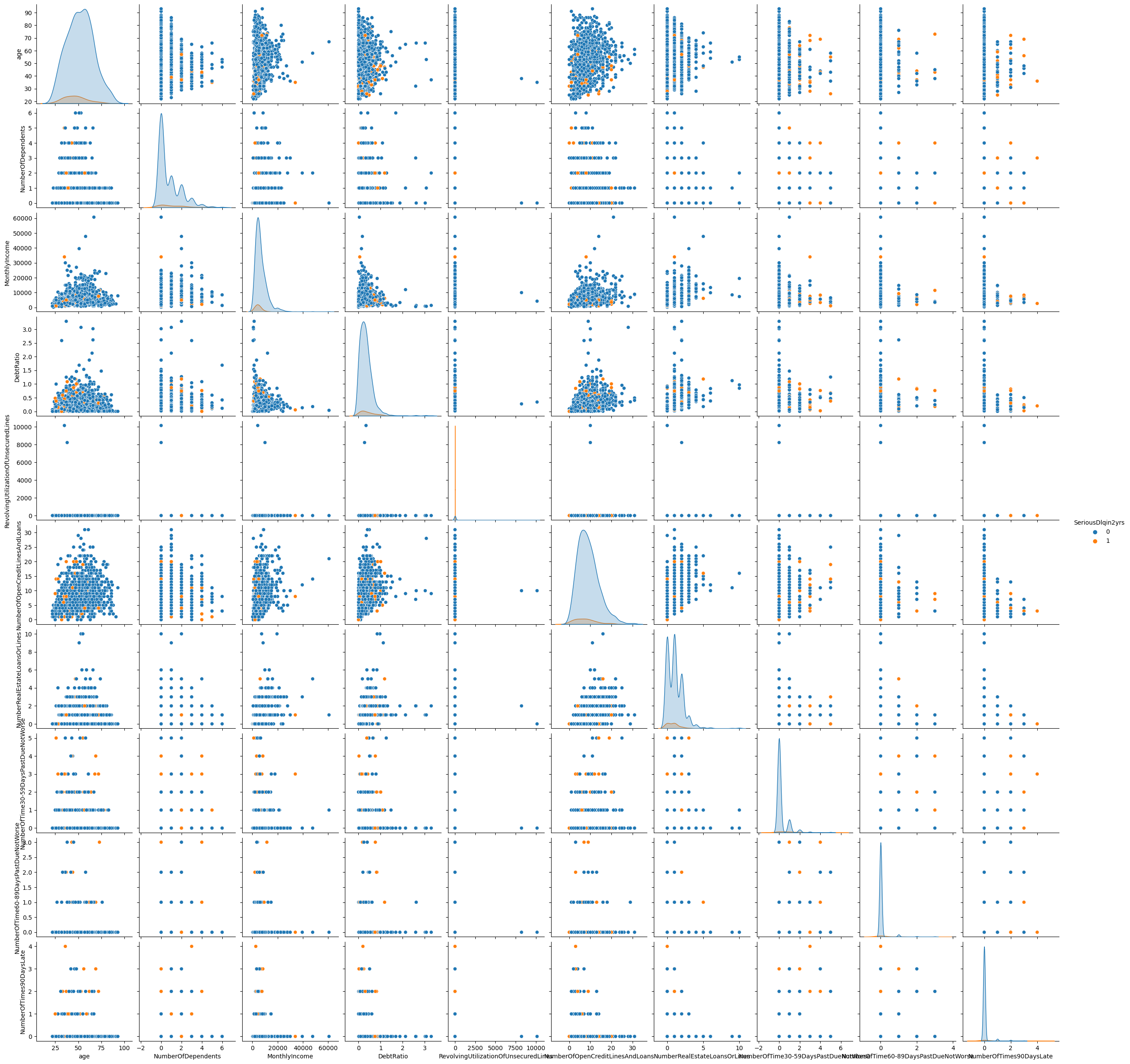
We have already looked at some variables selectively. To do it more broadly, we can look at the pair plot of the dataset. A pair plot shows the pairwise relationships between the variables in our dataset. On the diagonal, we are plotting the kernel density estimate
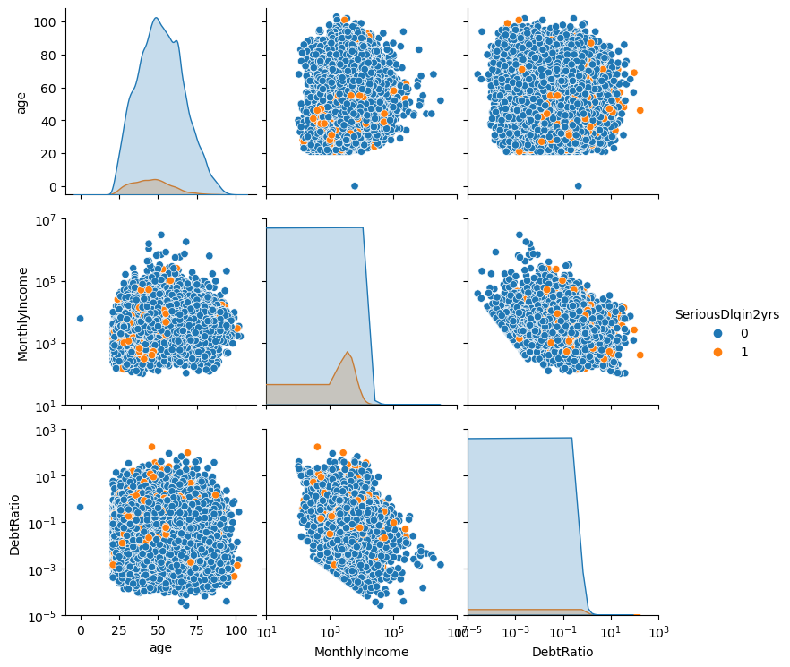
Note that we are plotting all variables in different colors based on whether our target variable SeriousDlqin2yrs is \(0\) or \(1\). Furthermore, since it is computationally quite demanding to create this plot, we have sampled only 1000 rows from the dataset. Since we have many variables, some of them with very skewed distributions, and also several discrete variables, it might make sense to look only at a subset
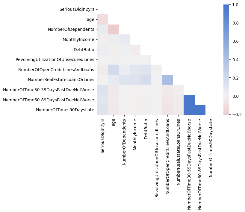
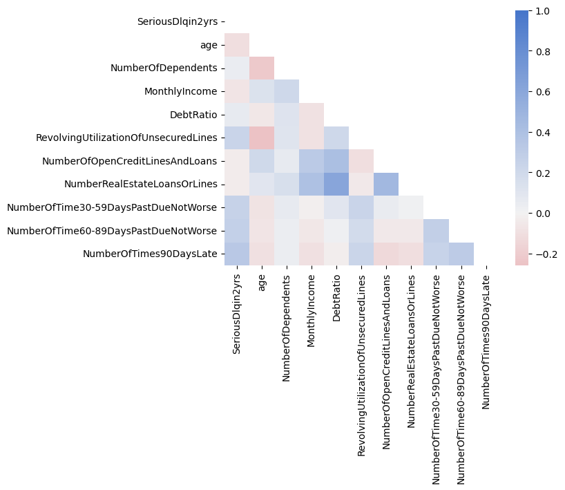
We can continue with the analysis of our dataset by looking at the correlation matrix of the variables in the dataset. We will calculate both the Pearson correlation (linear relationship) and the Spearman correlation (monotonic relationship) and create a heatmap of both correlation matrices
corr = df.corr() # Calculate the Pearson correlation (linear relationship)cmap = sns.diverging_palette(10, 255, as_cmap=True) # Create a color mapmask = np.triu(np.ones_like(corr, dtype=bool)) # Create a mask to only show the lower triangle of the matrixsns.heatmap(corr, cmap=cmap, vmax=1, center=0, mask=mask) # Create a heatmap of the correlation matrix (Note: vmax=1 makes sure that the color map goes up to 1 and center=0 are used to center the color map at 0)plt.show()
corr = df.corr('spearman') # Calculate the Spearman correlation (monotonic relationship)cmap = sns.diverging_palette(10, 255, as_cmap=True) # Create a color mapmask = np.triu(np.ones_like(corr, dtype=bool)) # Create a mask to only show the lower triangle of the matrixsns.heatmap(corr, cmap=cmap, vmax=1, center=0, mask=mask) # Create a heatmap of the correlation matrix (Note: vmax=1 makes sure that the color map goes up to 1 and center=0 are used to center the color map at 0)plt.show()
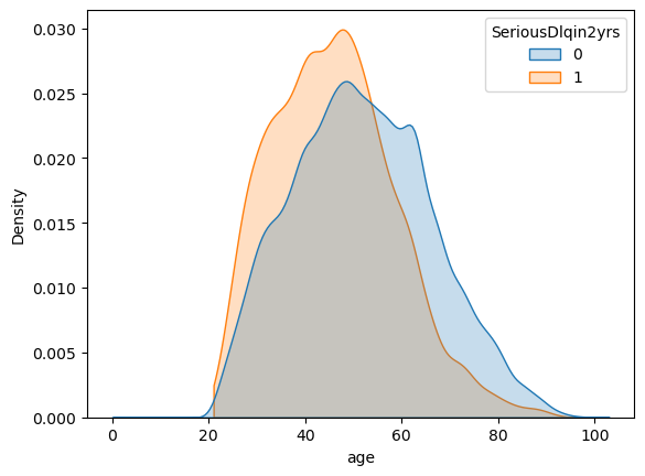
It seems that age is negatively correlated with default (SeriousDlqin2yrs) which we can also see in the kernel density estimate of the age variable
but then MonthlyIncome is also negatively correlated with default and with age. Thus, likely the relationship between age and default is driven by MonthlyIncome.
Furthermore, the variables NumberOfTime30-59DaysPastDueNotWorse, NumberOfTime60-89DaysPastDueNotWorse, and NumberOfTimes90DaysLate are highly correlated with each other and with the target variable SeriousDlqin2yrs. This is not surprising given that these variables are all related to the number of times a borrower has been past due on a loan payment. RevolvingUtilizationOfUnsecuredLines is also highly correlated with the target variable and with the number of times a borrower has been past due on a loan payment. This is also not surprising given that the RevolvingUtilizationOfUnsecuredLines is the ratio of the amount of money owed to the amount of credit available.
6.7 Implementation of Loan Default Prediction Models
We have explored our dataset and are now ready to implement machine learning algorithms for loan default prediction. Let’s start by importing the required libraries
6.7.1 Splitting the Data into Training and Test Sets
Before we can train a machine learning model, we need to split our dataset into a training set and a test set.
X = df.drop('SeriousDlqin2yrs', axis=1) # All variables except `SeriousDlqin2yrs`y = df['SeriousDlqin2yrs'] # Only SeriousDlqin2yrs
We follow Alonso Robisco and Carbó Martínez (2022) and use 80% of the data for training and 20% for testing. We will also set the stratify argument to y to make sure that the distribution of the target variable is the same in the training and test sets. Otherwise, we might randomly not have any defaulted loans in the test set, which would make it impossible to correctly evaluate our model.
To improve the performance of our machine learning model, we should scale the features. This is especially important for models that are sensitive to the scale of the features. We will use the MinMaxScaler class from the sklearn.preprocessing module to scale the features. The MinMaxScaler class scales the features so that they have a minimum of 0 and a maximum of 1.
def scale_features(scaler, df, col_names, only_transform=False):# Extract the features we want to scale features = df[col_names] # Fit the scaler to the features and transform themif only_transform: features = scaler.transform(features.values)else: features = scaler.fit_transform(features.values)# Replace the original features with the scaled features df[col_names] = featuresscaler = MinMaxScaler() scale_features(scaler, X_train, X_train.columns)scale_features(scaler, X_test, X_test.columns, only_transform=True)
Note that we have very skewed distributions for some variables in our dataset. This might make the MinMaxScaler less effective and there might be gains from more carefully scaling different variables. However, for the sake of simplicity, we will use the MinMaxScaler for all variables.
We have fully preprocessed and explored our dataset. The next step will be our main task: the implementation of machine learning algorithms for loan default prediction.
6.7.3 Evaluation Criertia
We will evaluate the performance of our machine-learning models using the following metrics:
Accuracy: The proportion of correctly classified instances
Precision: The proportion of true positive predictions among all positive predictions
Recall: The proportion of true positive predictions among all actual positive instances
ROC AUC: The area under the receiver operating characteristic curve
Furthermore, we will plot the ROC curve for each model to visualize the trade-off between the true positive rate and the false positive rate. To make the evaluation of our models more convenient, we will define a function that computes these metrics and plots the ROC curve for a given model
While we compute all of these metrics, we will focus on the ROC AUC score as our main evaluation metric.
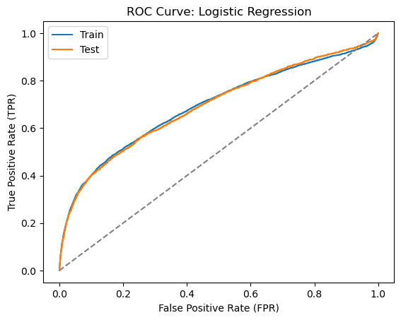
6.7.4 Logistic Regression
Let’s start with a simple logistic regression model. We will use the LogisticRegression class from the sklearn.linear_model module to train a logistic regression model. We will use the lbfgs solver and set the max_iter parameter to 5000 to make sure that the optimization algorithm converges. We will also set the penalty parameter to None to avoid regularization.
The model does not perform as well as what we have seen in previous lectures. The ROC AUC score is only around 0.7. Note again that the accuracy score is quite high but this is due to the imbalanced nature of the dataset.
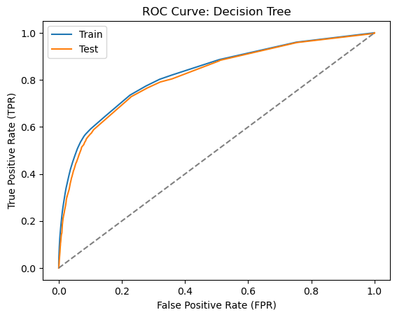
6.7.5 Decision Tree
Let’s now train a decision tree classifier. We will use the DecisionTreeClassifier class from the sklearn.tree module to train a decision tree classifier. We will set the max_depth parameter to 7 as in Alonso Robisco and Carbó Martínez (2022) to avoid overfitting.
The decision tree classifier performs better than the logistic regression model with a ROC AUC score of around 0.77. This is not surprising given that decision trees are more flexible models that can capture non-linear relationships in the data.
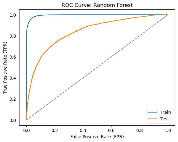
6.7.6 Random Forest
Let’s now train a random forest classifier. We will use the RandomForestClassifier class from the sklearn.ensemble module to train a random forest classifier. We will set the max_depth parameter to 20 and the n_estimators parameter to 100 as in Alonso Robisco and Carbó Martínez (2022).
This is a good example of the dangers of not using a test set for the evaluation of a model. The random forest classifier performs very well on the training set with a ROC AUC score of close to 1.0. However, it performs much worse on the test set with a ROC AUC score of around 0.83. Nevertheless, the random forest classifier still outperforms the logistic regression and decision tree classifiers.
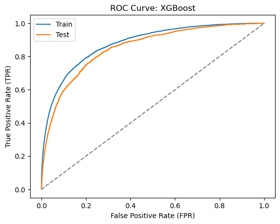
6.7.7 XGBoost
Let’s now train an XGBoost classifier. We will use the XGBClassifier class from the xgboost module to train an XGBoost classifier. We will set the max_depth parameter to 5 and the n_estimators parameter to 40 as in Alonso Robisco and Carbó Martínez (2022).
The XGBoost classifier performs quite well with an ROC AUC score of around 0.83. This is the best performance we have seen so far.
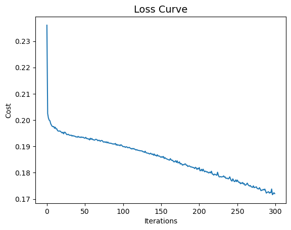
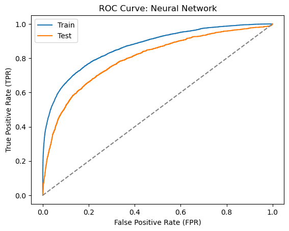
6.7.8 Neural Network
Finally, let’s train a neural network classifier. We will use the MLPClassifier class from the sklearn.neural_network module to train a neural network classifier. We will set the activation parameter to relu, the solver parameter to adam, and the hidden_layer_sizes parameter to (300,200,100) as in Alonso Robisco and Carbó Martínez (2022). We will also set the random_state parameter to 42 to make the results reproducible.
Since training the neural network classifier can take a long time, we have saved the trained model to a file called clf_nn.joblib. We can load the model from the file using the load function from the joblib module
clf_nn = load('clf_nn.joblib')
Let’s check the loss curve of the neural network classifier
But can we do better? Alonso Robisco and Carbó Martínez (2022) have also applied feature engineering to the dataset. Let’s see if we can improve the performance of our models by adding some additional features.
6.9 Feature Engineering and Model Improvement
We will add the square of each feature to the dataset to create additional features as in Alonso Robisco and Carbó Martínez (2022). We will use the assign method of the pandas DataFrame to add the squared features to the dataset
X2 = df.drop('SeriousDlqin2yrs', axis=1) # All variables except `SeriousDlqin2yrs`y2 = df['SeriousDlqin2yrs'] # Only SeriousDlqin2yrsX2 = X2.assign(**X2.pow(2).add_suffix('_sq')) # Add the squared features to the dataset
Then, we will split the dataset into a training set and a test set and scale the features
The models with the new features in the dataset perform better than the models without the new features. The random forest classifier and the XGBoost classifier have the best performance with ROC AUC scores of around 0.84 and 0.85, respectively.
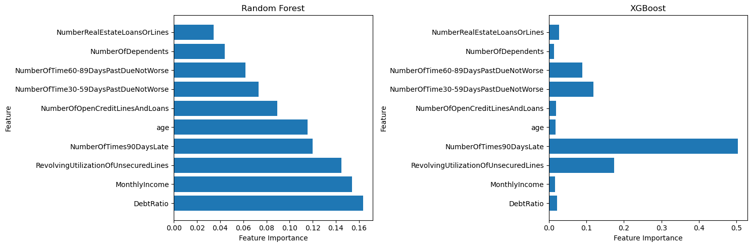
6.10 Feature Importance
We can also look at the feature importance of the random forest classifier and the XGBoost classifier to see which features are most important for predicting loan defaults. We will use the feature_importances_ attribute of the random forest classifier and the XGBoost classifier to get the feature importances
We have successfully implemented machine learning algorithms for loan default prediction. We have explored the dataset, preprocessed the data, trained several machine learning models, and evaluated their performance. We have also applied feature engineering to the dataset and improved the performance of the models. The random forest classifier and the XGBoost classifier have the best performance with ROC AUC scores of around 0.84 and 0.85, respectively. We have also looked at the feature importance of the random forest classifier and the XGBoost classifier to see which features are most important for predicting loan defaults.
Alonso Robisco, Andrés, and José Manuel Carbó Martínez. 2022. “Measuring the model risk-adjusted performance of machine learning algorithms in credit default prediction.”Financial Innovation 8 (1). https://doi.org/10.1186/s40854-022-00366-1.