4 Neural Networks
In this chapter, we have a look at neural networks which are a popular machine learning method. We will cover the basics of neural networks and how they can be trained.
4.1 What is a Neural Network?
Neural networks are at the core of many cutting-edge machine learning models. They can be used as both a supervised and unsupervised learning method. In this course, we will focus on their application in supervised learning where they are used for both regression and classification tasks. While they are conceptually not much more difficult to understand than decision trees, a neural network is not as easy to interpret as a decision tree. For this reason, they are often called black boxes, meaning that it is not so clear what is happening inside. Furthermore, neural networks tend to be more difficult to train and for tabular data, which is the type of structured data that you will typically encounter, gradient-boosted decision trees tend to perform better. Nevertheless, since neural networks are what enabled many of the recent advances in AI, they are an important topic to cover, even if it is only to better understand what has been driving recent innovations.
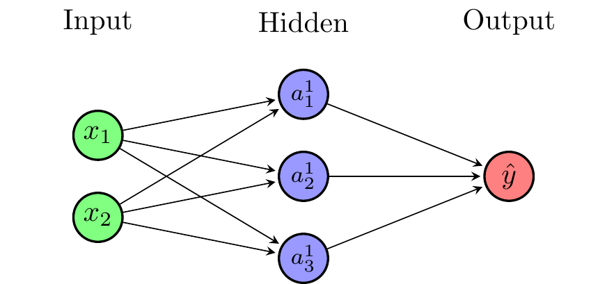
It is common to represent neural networks as directed graphs. Figure 4.1 shows a single-layer feedforward neural network with \(N=2\) inputs, \(M=3\) neurons in the hidden layer, and a single output. The input layer is connected to the hidden layer, which is connected to the output layer. For simplicity, we will only consider neural networks that are feedforward (i.e. their graphs are acyclical), with dense layers (i.e. each layer is fully connected to the previous), and without connections that skip layers.
As we will see later on, under certain (relatively weak) conditions
- Neural networks are universal approximators (can approximate any (Borel measurable) function)
- Neural networks break the curse of dimensionality (can handle very high dimensional functions)
This makes them interesting for a wide range of fields in economics, e.g., quantitative macroeconomics or econometrics. However, neural networks are not a magic bullet, and there are some downsides in terms of the large data requirements, interpretability and training difficulty.
4.1.1 Origins of the Term “Neural Network”
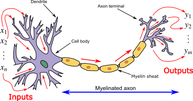
The term “neural network” originates in attempts to find mathematical representations of information processing in biological systems (Bishop 2006). The biological interpretation not very important for research anymore and one should not get too hung up on it. However, the interpretation can be useful when starting to learn about neural networks. Figure 4.2 shows a biological neuron.
4.2 An Artificial Neuron

Artificial neurons are the basic building blocks of neural networks. Figure 4.3 shows a single artificial neuron. The \(N\) inputs denoted \(x=(x_1,x_2,\ldots,x_N)'\) are linearly combined into \(z\) using weights \(w\) and bias \(b\)
\[z = b + \sum_{i=1}^N w_i x_i = \sum_{i=0}^N w_i x_i\]
where we defined an additional input \(x_0=1\) and \(w_0=b\).
The linear combination \(z\) is transformed using an activation function \(\phi(z)\).
\[a = \phi(z) = \phi\left( \sum_{i=0}^N w_i x_i \right)\]
The activation function introduces non-linearity into the neural network and allows it to learn highly non-linear functions. The particular choice of activation function depends on the application.
This should look familiar to you already. If we set \(\phi(z)=z\), we get a linear regression model and if we set \(\phi(z)=\frac{1}{1+e^{-z}}\), we get a logistic regression model. This is because the basic building block, the artificial neuron, is a generalized linear model.
4.2.1 Activation Functions
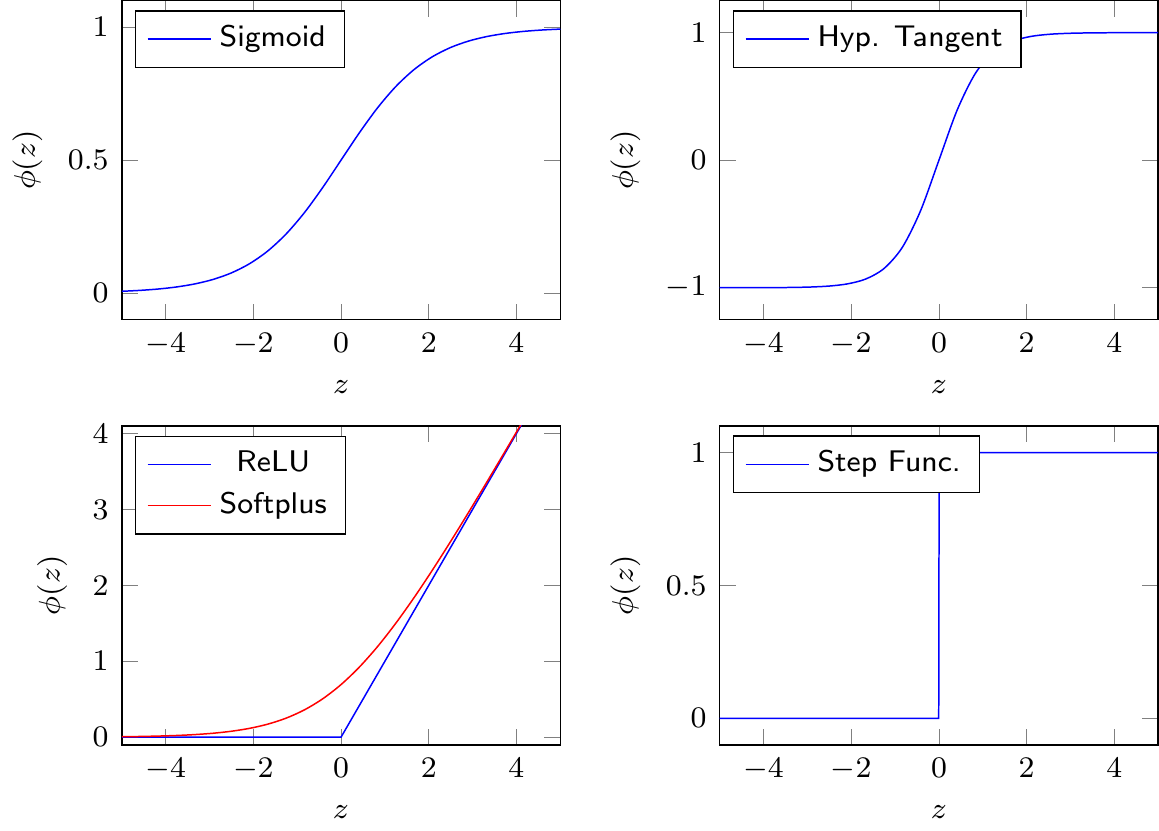
Common activation functions include
- Sigmoid: \(\phi(z) = \frac{1}{1+e^{-z}}\)
- Hyperbolic tangent: \(\phi(z) = tanh(z)\)
- Rectified linear unit (ReLU): \(\phi(z) = \max(0,z)\)
- Softplus: \(\phi(z) =\log(1+e^{z})\)
ReLU has become popular in deep neural networks in recent years because of its good performance in these applications. Since economic problems usually involve smooth functions, softplus can be a good alternative.
4.2.2 A Special Case: Perceptron
Perceptrons were developed in the 1950s and have only one artificial neuron. Perceptrons use a step function as an activation function
\[\phi(z) = \begin{cases} 1 & \text{if } z \geq 0\\ 0 & \text{otherwise}\,, \end{cases}\]
Perceptrons can be used for basic classification. However, the step function is usually not used in neural networks because it is not differentiable at \(z=0\) and zero everywhere else. This makes it unsuitable for the back-propagation algorithm, which is used for determining the network weights.
Mini-Exercise
What would the decision boundary of a perceptron look like if we have two inputs \(x_1\) and \(x_2\) and the weights \(w_1=1\), \(w_2=1\), and \(b=-1\)?
4.3 Building a Neural Network from Artificial Neurons
We can build a neural network by stacking multiple artificial neurons. For this reason, it is sometimes also called a multilayer perceptron (MLP). A single-layer neural network is a linear combination of \(M\) artificial neurons \(a_j\)
\[ a_j = \phi(z_j) = \phi\left( b_{j}^{1} + \sum_{i=1}^N w_{ji}^{1} x_i \right)\]
with the output defined as
\[ g(x ; w) = b^{2}+\sum_{j=1}^{M} w_{j}^{2} a_j\]
where \(N\) is the number of inputs, \(M\) is the number of neurons in the hidden layer, and \(w\) are the weights and biases of the network. The width of the neural network is \(M\).
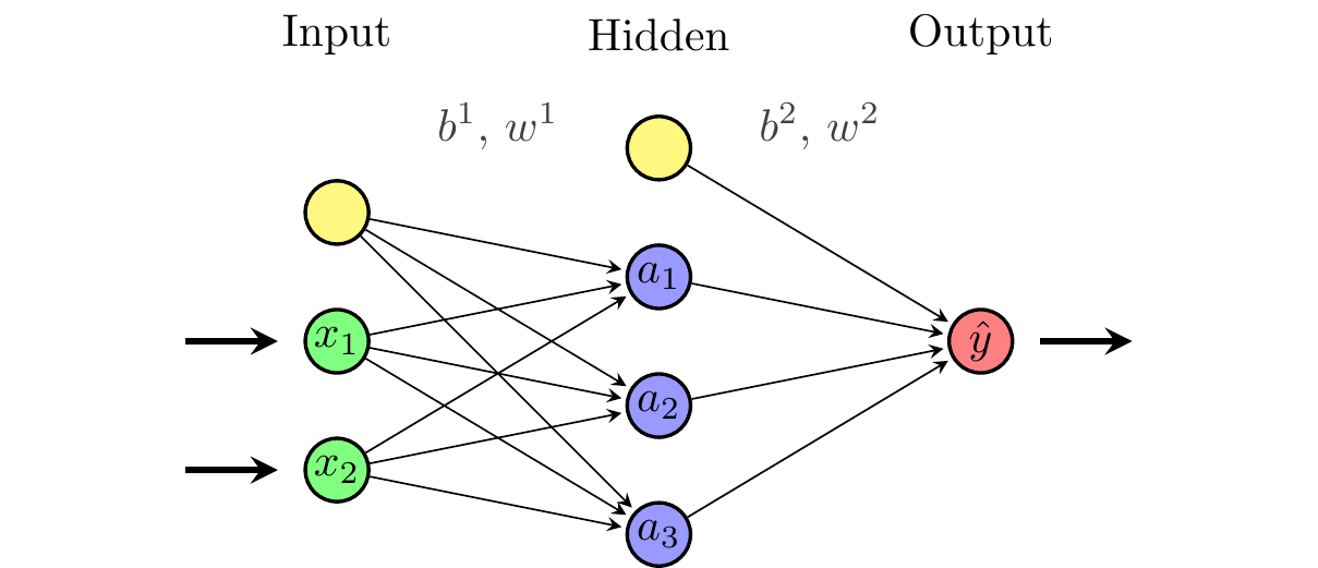
Figure 4.5 shows a single-layer feedforward neural network with \(N=2\) inputs, \(M=3\) neurons in the hidden layer, and a single output. Note that the biases can be thought of as additional weights that are multiplied by a constant input of 1.
4.4 Relation to Linear Regression
Note that if we use a linear activation function, e.g. \(\phi(x)=x\), the neural network collapses to a linear regression
\[ y \cong g(x ; w) = \tilde{w}_{0} +\sum_{i=1}^{N} \tilde{w}_{i} x_{i}\]
with appropriately defined regression coefficients \(\tilde{w}\).
Recall that in our description of Figure 2.2 we argued that a machine learning algorithm would automatically turn the slider to find the best fit. This is exactly what the training algorithm has to do to train a neural network.
4.5 A Simple Example
Suppose we want to approximate \(f(x)=exp(x)-x^3\) with 3 neurons. The approximation might be
\[\hat{f}(x)=a_1+a_2-a_3\]
where
\[a_1=max(0,-3x-1.5)\]
\[a_2=max(0,x+1)\]
\[a_3=max(0,3x-3)\]
Our neural network in this case uses ReLU activation functions and has all weights equal to one in the output layer. Figure 4.6 shows the admittedly poor approximation of \(f(x)\) by \(\hat{f}(x)\) using this neural network. Given the piecewise linear nature of the ReLU activation function, the approximation is not very good. However, with more neurons, we could get a better approximation.
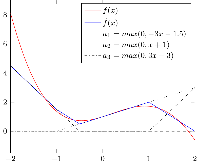
Figure 4.7 shows an interactive version of Figure 4.6 where you can adjust the weights of the neural network to approximate a simple dataset. As you can see, it is quite tricky to find parameters that approximate the function well. This is where the training algorithm comes in. It will automatically adjust the weights to minimize a loss function.
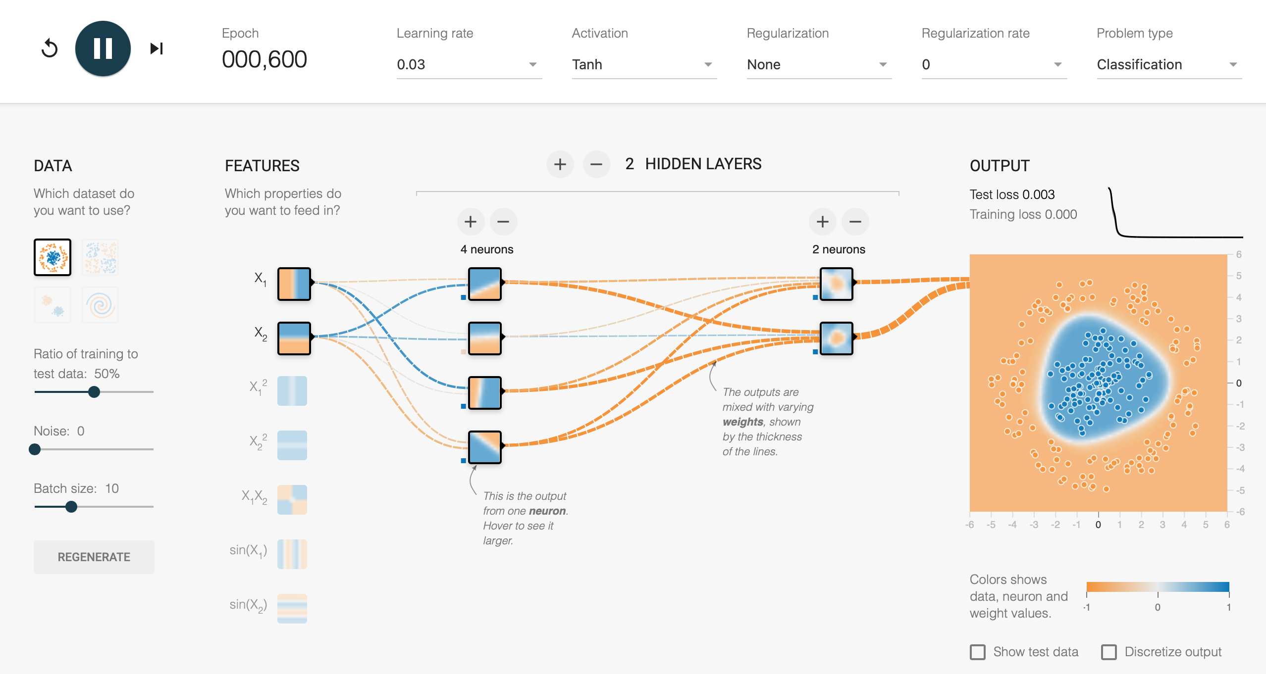
TensorFlow Playground
If you want to play around with neural networks, you can use the TensorFlow Playground: https://playground.tensorflow.org. It is a web-based tool that allows you to experiment with neural networks and see how they learn. Figure 4.8 shows the interface of the TensorFlow Playground.
4.6 Deep Neural Networks
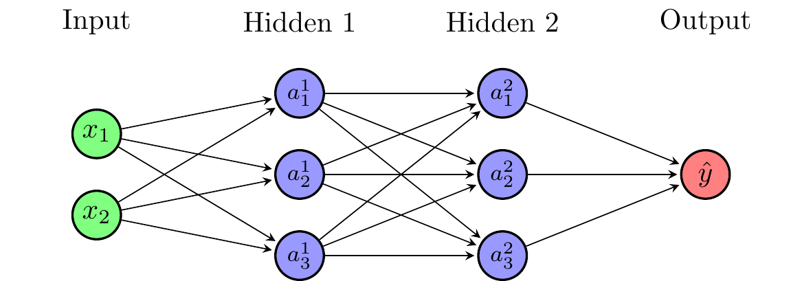
Deep neural networks have more than one hidden layer. The number of hidden layers is also called the depth of the neural network. Deep neural networks can learn more complicated things. For simple function approximation, a single hidden layer is sufficient. Figure 4.9 shows a deep neural network with two hidden layers.
The first hidden layer consists of \(M_1\) artificial neurons with inputs \(x_1,x_2,\ldots,x_N\)
\[a_j^{1} = \phi\left( b_{j}^{1} + \sum_{i=1}^N w_{ji}^{1} x_i \right)\]
The second hidden layer consists of \(M_2\) artificial neurons with inputs \(a_1^{1},a_2^{1},\ldots,a_{M_1}^{1}\)
\[a_k^{2} = \phi\left( b_{k}^{2} + \sum_{j=1}^{M_1} w_{kj}^{2} a_j^{1} \right)\]
After \(Q\) hidden layers, the output is defined as
\[y \cong g(x ; w) = b^{Q+1}+\sum_{j=1}^{M_{Q}} w_{j}^{Q+1} a_j^{Q}\]
Note that the activation functions do not need to be the same everywhere. In principle, we could vary the activation functions even within a layer.
4.7 Universal Approximation and the Curse of Dimensionality
Recall that we want to approximate an unknown function in supervised learning tasks
\[y = f(x)\]
where \(y=(y_1,y_2,\ldots,y_K)'\) and \(x=(x_1,x_2,\ldots,x_N)'\) are vectors. The function \(f(x)\) could stand for many different functions in economics (e.g. a value function, a policy function, a conditional expectation, a classifier, \(\ldots\)).
It turns out that neural networks are universal approximators and break the curse of dimensionality. The universal approximation theorem by Hornik, Stinchcombe, and White (1989) states:
A neural network with at least one hidden layer can approximate any Borel measurable function mapping finite-dimensional spaces to any desired degree of accuracy.
Breaking the curse of dimensionality (Barron, 1993)
A one-layer NN achieves integrated square errors of order \(O(1/M)\), where \(M\) is the number of nodes. In comparison, for series approximations, the integrated square error is of order \(O(1/(M^{2/N}))\) where \(N\) is the dimensions of the function to be approximated.
4.8 Training a Neural Network: Determining Weights and Biases
We have not yet discussed how to determine the weights and biases. The weights and biases \(w\) are selected to minimize a loss function
\[E(w; X, Y) = \frac{1}{N} \sum_{n=1}^{N} E_n(w; x_n, y_n)\]
where \(N\) refers to the number of input-output pairs that we use for training and \(E_n(w; x_n, y_n)\) refers to the loss of an individual pair \(n\).
For notational simplicity, I will write \(E(w)\) and \(E_n(w)\) in the following or in some cases even omit argument \(w\).
4.8.1 Choice of Loss Function
The choice of loss function depends on the problem at hand. In regressions, one often uses a mean squared error (MSE) loss
\[E_n(w; x_n, y_n) = \frac{1}{2} \left\|g\left(x_{n}; w\right)-y_{n}\right\|^{2}\]
In classification problems, one often uses a cross-entropy loss
\[E_n(w; x_n, y_n) = \sum_{k=1}^K y_{nk} \log(g_k(x_n;w))\]
where \(k\) refers to \(k\)th class (or \(k\)th element) in the output vector.
4.8.2 Gradient Descent
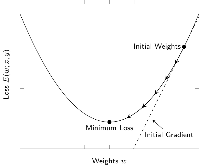
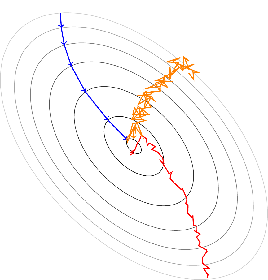
The weights and biases are determined by minimizing the loss function using a gradient descent algorithm. The basic idea is to compute how the loss changes with the weights \(w\) and step into the direction that reduces the loss. Figure 4.10 shows a simple example of a loss function and the gradient descent algorithm. The basic steps of the algorithm are
- Initialize weights (e.g. draw from Gaussian distribution)
\[w^{(0)} \sim N(0,I)\]
- Compute the gradient of the loss function with respect to weights
\[\nabla E(w^{(i)}) = \frac{1}{N}\sum_{n=1}^N \nabla E_n\left(w^{(i)}\right)\]
- Update weights (make a small step in the direction of the negative gradient)
\[w^{(i+1)} = w^{(i)} - \eta \nabla E\left(w^{(i)}\right)\]
where \(\eta>0\) is the learning rate.
- Repeat Steps 2 and 3 until a terminal condition (e.g. fixed number of iterations) is reached.
If we use the batch gradient descent algorithm described above, we might get stuck in a local minimum. To avoid this, we can use
Stochastic gradient descent: Use only a single observation to compute the gradient and update the weights for each observation
\[w^{(i+1)} = w^{(i)} - \eta \nabla E_n\left(w^{(i)}\right)\]
Minibatch gradient descent: Use a small batch of observations (e.g. 32) to compute the gradient and update the weights for each minibatch
These algorithms are less likely to get stuck in a shallow local minimum of the loss function because they are “noisier”. Figure 4.11 shows a comparison of the different gradient descent algorithms. Minibatch gradient descent is probably the most commonly used and is also what we will be using in our implementation in Python.
4.8.3 Backpropagation Algorithm
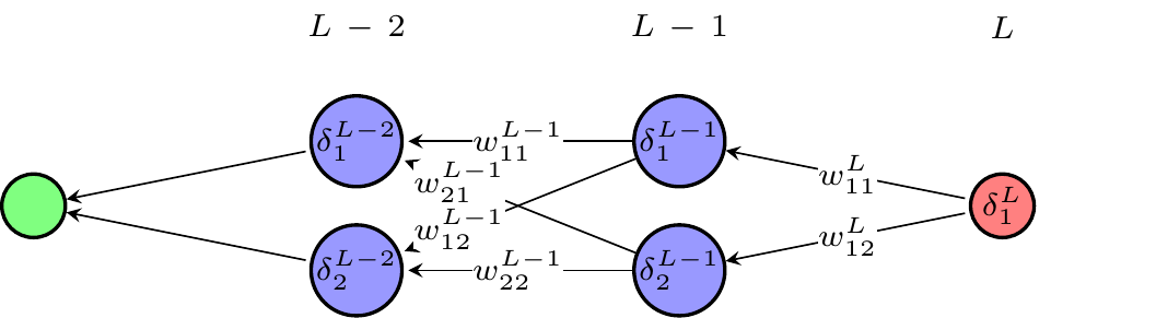
Computing the gradient seems to be a daunting task since a weight in the first layer in a deep neural network affects the loss function potentially through thousands of “paths”. The backpropagation algorithm (Rumelhart et al., 1986) provides an efficient way to evaluate the gradient. The basic idea is to go backward through the network to evaluate the gradient as shown in Figure 4.12. If you are interested in the details, I recommend reading the notes by Nielsen (2019).
4.9 Practical Considerations
From a practical perspective, there are many more things to consider. Often times it’s beneficial to do some (or all) of the following
- Input/output normalization: (e.g. to have unit variance and mean zero) can improve the performance of the NN
- Check for overfitting: by splitting the dataset into a training dataset and a test dataset
- Regularization: to avoid overfitting (e.g. add a term to lose function that penalizes large weights)
- Adjust the learning rate: \(\eta\) during training
We have already discussed some of these topics in the context of other machine learning algorithms.
4.10 Python Implementation
Let’s have a look at how to implement a neural network in Python.
4.10.1 Implementing the Feedforward Part of a Neural Network
As a small programming exercise and to improve our understanding of neural networks, let’s implement the feedforward part of a neural network from scratch. We will have to calculate the output of the network for some given weights and biases, as well as some inputs. Let’s start by importing the necessary libraries
import numpy as npNext, we define the activation function for which we use the sigmoid function
def activation_function(x):
    return 1/(1+np.exp(-x)) # sigmoid function
Now, we define the feedforward function which calculates the output of the neural network given some inputs, weights, and biases. The function takes the inputs, weights, and biases as arguments and returns the output of the network
def feedforward(inputs, w1, w2, b1, b2):

    # Compute the pre-activation values for the first layer
    z = b1 + np.matmul(w1, inputs)

    # Compute the post-activation values for the first layer
    a = activation_function(z)

    # Combine the post-activation values of the first layer to an output
    g = b2 + np.matmul(w2, a)

    return g
Mathematically, the function computes the following
\(z = b^{1} + w^1 x\)
\(a = \phi(z)\)
\(g = b^2 + w^2 a\)
and returns \(g\) at the end. We have written this using matrix notation to make it more compact. Remember that node \(j\) in the hidden layer is given by
\(z_j = b_{j}^{1} + \sum_{i=1}^N w_{ji}^{1} x_i\)
\(a_j = \phi(z_j)\)
and the output of the network is given by
\(g(x ; w) = b^{2}+\sum_{j=1}^{M} w_{j}^{2} a_j.\)
Let’s test the function with some example inputs, weights and biases
# Define the weights and biases
w1 = np.array([[0.1, 0.2], [0.3, 0.4]]) # 2x2 matrix
w2 = np.array([0.5, 0.6]) # 1-d vector
b1 = np.array([0.1, 0.2]) # 1-d vector
b2 = 0.3

# Define the inputs
inputs = np.array([1, 2]) # 1-d vector

# Compute the output of the network
feedforward(inputs, w1, w2, b1, b2)np.float64(1.0943291429384328)To operationalize this, we would also need to define a loss function and an optimization algorithm to update the weights and biases. However, this is beyond the scope of this course.
4.10.2 Using Neural Networks in Sci-Kit Learn
Sci-kit learn provides a simple interface to use neural networks. However, it is not as flexible as the more commonly used PyTorch or TensorFlow. We can reuse the dataset of credit card transactions from Kaggle.com to demonstrate how to use neural networks in scikit-learn.
import pandas as pd
import numpy as np
import matplotlib.pyplot as plt
import seaborn as sns
from sklearn.preprocessing import StandardScaler, MinMaxScaler
from sklearn.neural_network import MLPClassifier
from sklearn.model_selection import train_test_split
from sklearn.metrics import confusion_matrix, accuracy_score, roc_auc_score, recall_score, precision_score, roc_curve
pd.set_option('display.max_columns', 50) # Display up to 50 columns
from io import BytesIO
from urllib.request import urlopen
from zipfile import ZipFile
import os.path

# Check if the file exists
if not os.path.isfile('data/card_transdata.csv'):

    print('Downloading dataset...')

    # Define the dataset to be downloaded
    zipurl = 'https://www.kaggle.com/api/v1/datasets/download/dhanushnarayananr/credit-card-fraud'

    # Download and unzip the dataset in the data folder
    with urlopen(zipurl) as zipresp:
        with ZipFile(BytesIO(zipresp.read())) as zfile:
            zfile.extractall('data')

    print('DONE!')

else:

    print('Dataset already downloaded!')

# Load the data
df = pd.read_csv('data/card_transdata.csv')

# Split the data into training and test sets
X = df.drop('fraud', axis=1) # All variables except `fraud`
y = df['fraud'] # Only our fraud variables
X_train, X_test, y_train, y_test = train_test_split(X, y, stratify=y, test_size = 0.3, random_state = 42)

# Scale the features
def scale_features(scaler, df, col_names, only_transform=False):

    # Extract the features we want to scale
    features = df[col_names]

    # Fit the scaler to the features and transform them
    if only_transform:
        features = scaler.transform(features.values)
    else:
        features = scaler.fit_transform(features.values)

    # Replace the original features with the scaled features
    df[col_names] = features

col_names = ['distance_from_home', 'distance_from_last_transaction', 'ratio_to_median_purchase_price']
scaler = StandardScaler()
scale_features(scaler, X_train, col_names)
scale_features(scaler, X_test, col_names, only_transform=True)
Dataset already downloaded!Recall that the target variable \(y\) is fraud, which indicates whether the transaction is fraudulent or not. The other variables are the features \(x\) of the transactions.
To use a neural network for a classification task, we can use the MLPClassifier class from scikit-learn. The following code snippet shows how to use a neural network with one hidden layer with 16 nodes
clf = MLPClassifier(hidden_layer_sizes=(16,), random_state=42, verbose=False).fit(X_train, y_train)If you would like to use a neural network with multiple hidden layers, you can specify the number of nodes per hidden layer using the hidden_layer_sizes parameter. For example, the following code snippet shows how to use a neural network with two hidden layers, one with 5 nodes and the other with 4 nodes
clf = MLPClassifier(alpha=1e-5, hidden_layer_sizes=(5,4), activation='logistic', random_state=42).fit(X_train, y_train)Note that the alpha parameter specifies the regularization strength, the activation parameter specifies the activation function (by default it uses relu) and the random_state parameter specifies the seed for the random number generator (useful for reproducible results).
We can check the loss curve to see how the neural network loss declined during training
plt.plot(clf.loss_curve_)
plt.title("Loss Curve", fontsize=14)
plt.xlabel('Iterations')
plt.ylabel('Cost')
plt.show()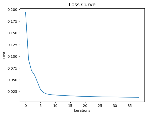
We can then use the same way to evaluate the neural network performance as we did for the other ML models
y_pred = clf.predict(X_test)
y_proba = clf.predict_proba(X_test)

print(f"Accuracy: {accuracy_score(y_test, y_pred)}")
print(f"Precision: {precision_score(y_test, y_pred)}")
print(f"Recall: {recall_score(y_test, y_pred)}")
print(f"ROC AUC: {roc_auc_score(y_test, y_proba[:, 1])}")
Accuracy: 0.9955266666666667
Precision: 0.971747127308582
Recall: 0.9772319896266352
ROC AUC: 0.9996638991577014The neural network performs substantially better than the logistic regression. As in the case of the tree-based methods, the ROC AUC score is much closer to the maximum value of 1 and we have an almost perfect classifier
# Compute the ROC curve
fpr, tpr, thresholds = roc_curve(y_test, y_proba[:, 1])

# Plot the ROC curve
plt.plot(fpr, tpr)
plt.plot([0, 1], [0, 1], linestyle='--', color='grey')
plt.xlabel('False Positive Rate (FPR)')
plt.ylabel('True Positive Rate (TPR)')
plt.title('ROC Curve')
plt.show()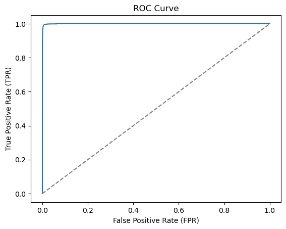
Let’s also check the confusion matrix to see where we still make mistakes
conf_mat = confusion_matrix(y_test, y_pred, labels=[1, 0]).transpose() # Transpose the sklearn confusion matrix to match the convention in the lecture
sns.heatmap(conf_mat, annot=True, cmap='Blues', fmt='g', xticklabels=['Fraud', 'No Fraud'], yticklabels=['Fraud', 'No Fraud'])
plt.xlabel("Actual")
plt.ylabel("Predicted")
plt.show()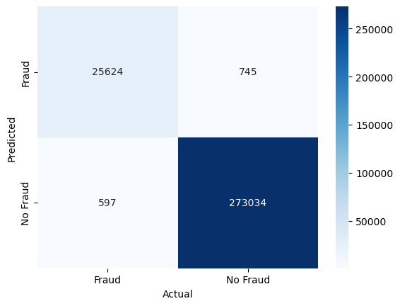
There are around 270 false negatives, i.e., a fraudulent transaction that we did not detect. There are also around 980 false positives, i.e., “false alarms”, where non-fraudulent transactions were classified as fraudulent.
4.10.3 Using Neural Networks in PyTorch
While it is possible to use neural networks in scikit-learn, it is more common to use PyTorch or TensorFlow for neural networks. PyTorch is a popular deep-learning library that is widely used in academia and industry. In this section, we will show how to use PyTorch to build a simple neural network for the same credit card fraud detection task.
Feel Free to Skip This Section
This section might be a bit more challenging than what we have looked at previously. If you think that you are not ready for this, feel free to skip this section. This is mainly meant to be a starting point for those who are interested in learning more about neural networks.
For a more in-depth introduction to PyTorch, I recommend that you check out the official PyTorch tutorials. This section, in particular, builds on the Learning PyTorch with Examples tutorial.
Let’s start by importing the necessary libraries
import torch
from torch.utils.data import DataLoader, TensorDataset
Then, let’s prepare the data for PyTorch. We need to convert the data in our DataFrame to PyTorch tensors
X_train_tensor = torch.tensor(X_train.values, dtype=torch.float32)
y_train_tensor = torch.tensor(y_train.values, dtype=torch.long)
Note that we also converted the input values to float32 for improved training speed and the target values to long which is a type of integer (remember our target y can only take values zero or one). Next, we need to create a DataLoader object to load the data in mini-batches during the training process
dataset = TensorDataset(X_train_tensor, y_train_tensor)
dataloader = DataLoader(dataset, batch_size=200, shuffle=True)
dataset_size = len(dataloader.dataset)
Next, we define the neural network model using the nn module from PyTorch
model = torch.nn.Sequential(
    torch.nn.Linear(7, 16), # 7 input features, 16 nodes in the hidden layer
    torch.nn.ReLU(),        # ReLU activation function
    torch.nn.Linear(16, 2) # 16 nodes in the hidden layer, 2 output nodes (fraud or no fraud)
)
We also need to define the loss function and the optimizer. We will use the cross-entropy loss function and the Adam optimizer
loss_fn = torch.nn.CrossEntropyLoss()
optimizer = torch.optim.Adam(model.parameters(), lr=1e-3, weight_decay=1e-5) # Adam optimizer with learning rate of 0.001 and L2 regularization (analogous to alpha in scikit-learn)
We can now train the neural network using the following code snippet
for epoch in range(80):

    # Loop over batches in an epoch using DataLoader
    for id_batch, (X_batch, y_batch) in enumerate(dataloader):

        # Compute the predicted y using the neural network model with the current weights
        y_batch_pred = model(X_batch)

        # Compute the loss
        loss = loss_fn(y_batch_pred, y_batch)

        # Reset the gradients of the loss function to zero
        optimizer.zero_grad()

        # Compute the gradient of the loss with respect to model parameters
        loss.backward()

        # Update the weights by taking a "step" in the direction that reduces the loss
        optimizer.step()

    if epoch % 10 == 9:
        print(f"Epoch {epoch} loss: {loss.item():>7f}")
Epoch 9 loss: 0.024499
Epoch 19 loss: 0.008713
Epoch 29 loss: 0.016122
Epoch 39 loss: 0.007585
Epoch 49 loss: 0.005461
Epoch 59 loss: 0.020942
Epoch 69 loss: 0.016723
Epoch 79 loss: 0.007653Note that here we are updating the model weights for each mini-batch in the dataset and go over the whole dataset 80 times (epochs). We print the loss every epoch to see how the loss decreases over time.
The following snippet shows how to use full-batch gradient descent instead of mini-batch gradient descent
for epoch in range(2000):

    # Compute the predicted y using the neural network model with the current weights
    y_epoch_pred = model(X_train_tensor)

    # Compute the loss
    loss = loss_fn(y_epoch_pred, y_train_tensor)

    # Reset the gradients of the loss function to zero
    optimizer.zero_grad()

    # Compute the gradient of the loss with respect to model parameters
    loss.backward()

    # Update the weights by taking a "step" in the direction that reduces the loss
    optimizer.step()

    # Print the loss every 100 epochs
    if epoch % 100 == 99:
        print(f"Epoch {epoch} loss: {loss.item():>7f}")
Epoch 99 loss: 0.009982
Epoch 199 loss: 0.009945
Epoch 299 loss: 0.009928
Epoch 399 loss: 0.009920
Epoch 499 loss: 0.009914
Epoch 599 loss: 0.009910
Epoch 699 loss: 0.009907
Epoch 799 loss: 0.009904
Epoch 899 loss: 0.009901
Epoch 999 loss: 0.009899
Epoch 1099 loss: 0.009897
Epoch 1199 loss: 0.009895
Epoch 1299 loss: 0.009893
Epoch 1399 loss: 0.009891
Epoch 1499 loss: 0.009890
Epoch 1599 loss: 0.009888
Epoch 1699 loss: 0.009886
Epoch 1799 loss: 0.009885
Epoch 1899 loss: 0.009883
Epoch 1999 loss: 0.009881Note that in this version we are updating the model weights 2000 times (epochs) and printing the loss every 100 epochs. We can now evaluate the model on the test set
X_test_tensor = torch.tensor(X_test.values, dtype=torch.float32)
y_pred = torch.argmax(model(X_test_tensor), dim=1).numpy()

print(f"Accuracy: {accuracy_score(y_test, y_pred)}")
print(f"Precision: {precision_score(y_test, y_pred)}")
print(f"Recall: {recall_score(y_test, y_pred)}")
Accuracy: 0.9965833333333334
Precision: 0.9775587566338135
Recall: 0.9834865184394188Note that for simplicity we are reusing the sci-kit learn metrics to evaluate the model.
However, our neural network trained in PyTorch does not perform exactly the same as the neural network trained in scikit-learn. This is likely because of different hyperparameters or different initializations of the weights. In practice, it is common to experiment with different hyperparameters to find the best model or to use grid search and cross-validation to try many values and find the best-performing ones.
4.10.4 Conclusions
In this chapter, we have learned about neural networks, which are the foundation of deep learning. We have seen how to implement parts of a simple neural network from scratch and how to use neural networks in scikit-learn and PyTorch.